Detailed example
To illustrate platerecipy's functionalities on a reproducible input, let's work
with an input field generated by a pseudorandom sum of spherical harmonics:
 1
 2
 3
 4
 5
 6
 7
 8
 9
10
11
12
13
14
15
16
17
18
19
20
21
22
23
24
25 | import numpy as np
def generate_sample_input(lrange=(1, 4), rng_seed=111, npoints=100_000):
from scipy.special import sph_harm_y
from scipy.ndimage import laplace
thetas, phis = np.meshgrid(
np.linspace(0, np.pi, 300),
np.linspace(-np.pi, np.pi, 600),
indexing='ij'
)
rng = np.random.default_rng(rng_seed)
F = 0
for l in range(lrange[0], lrange[1]):
for m in range(-l, l+1):
F += (rng.uniform()-0.25) * sph_harm_y(l, m, thetas, phis).real
F = laplace(np.abs(F))
rand_data = rng.choice(thetas.size, size=npoints, replace=False)
data_phis = phis.ravel()[rand_data]
data_thetas = thetas.ravel()[rand_data]
data_F = F.ravel()[rand_data]
data_xs = np.sin(data_thetas)*np.cos(data_phis)
data_ys = np.sin(data_thetas)*np.sin(data_phis)
data_zs = np.cos(data_thetas)
return data_xs, data_ys, data_zs, data_F
|
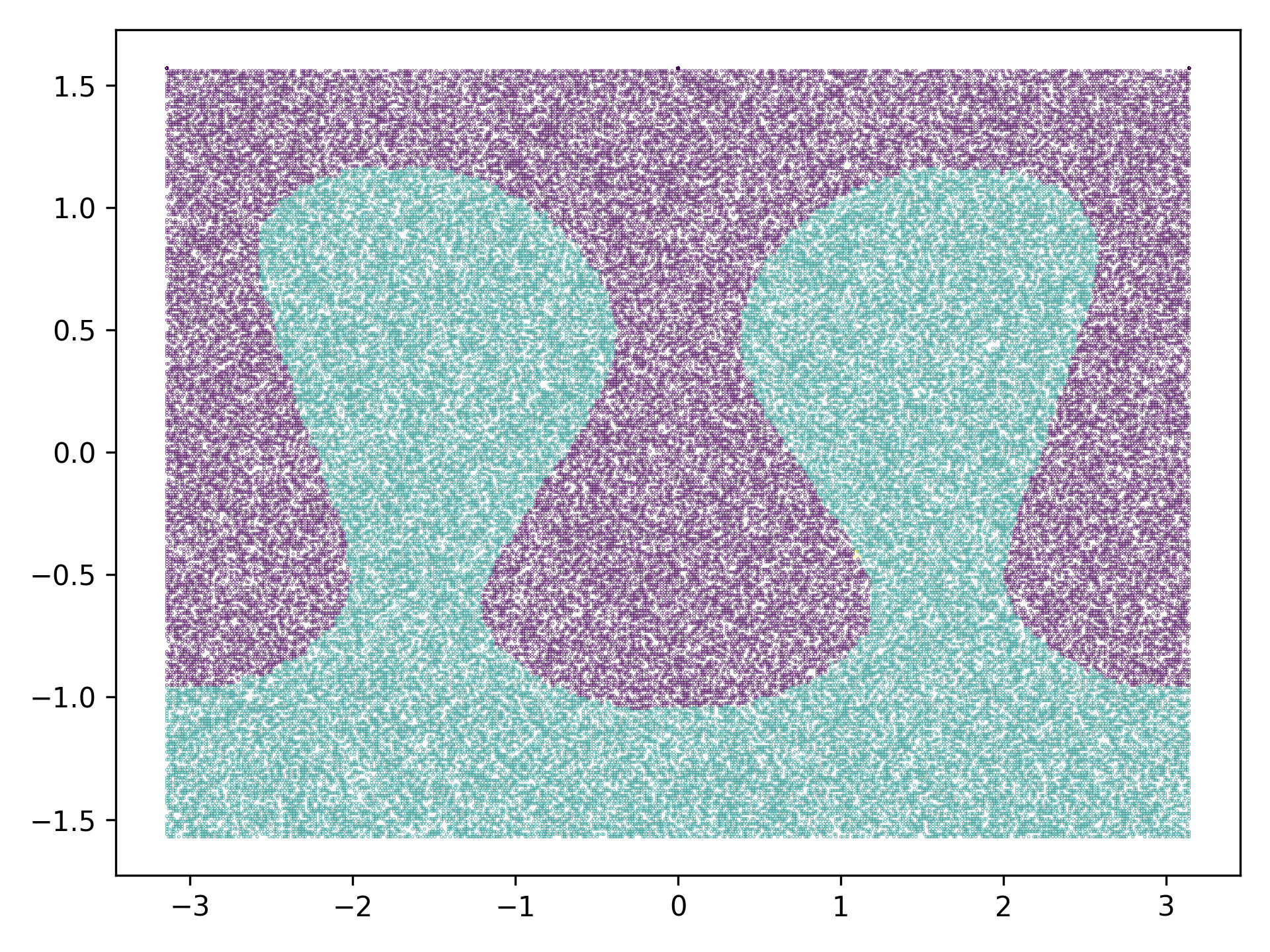
generate_sample_input function now will generate an ungridded set of 100,000 points that
are randomly sampled from the surface of a sphere with unit radius. We store the
data points as:
| data_xs, data_ys, data_zs, data_F = generate_sample_input()
|
data_xs, data_ys, and data_zs are the Cartesian coordinates of each
point with field value data_F. Up to this point, we've merely generated a set
of points with no inherent structure.
Now, let's use platerecipy's SphericalGrid object to generate a grid and
interpolate field values:
| from platerecipy.grid import SphericalGrid
# initializing a grid base on input coordinates
grid = SphericalGrid(data_xs, data_ys, data_zs)
# interpolating the input data
field1 = grid.interpolate_field(data_F)
|
Coordinate compatibility
For optimization purposes, grid.interpolate_field() can only accept an input
argument (data_F) that has coordinates identical to what used to initialize
the grid object.
Now, we can define a PlateModel object on our SphericalGrid:
| from platerecipy.model import PlateModel
# initializing a plate model
model = PlateModel(grid)
# stacking our interpolated field
model.stack_field(field1)
# additional fields can be stacked here
|
Finally, we can use our model to find plates by specifying our plate detection
parameters of choice:
| model.find_plates(
boundary_quantile = 0.95,
RW_beta = 100.0,
)
|
Field stacking
Once the find_plates() method is called, no more fields can be stacked.
Now, the following 2D arrays are accessible via the model object:
| model.stacked_field # the normalized [0, 1] stacked field
model.markers # segmentation markers as a diagnostic tool
model.plate_IDs # plate IDs
model.ID_probs # the probability field
|
grid object. This is
important as one can easy use the grid object to retrieve:
| grid.xs # Cartesian x-coordinate
grid.ys # Cartesian y-coordinate
grid.zs # Cartesian z-coordinate
grid.thetas # Spherical colatiude [0, pi]
grid.phis # Spherical azimuth [-pi, pi]
grid.r # Radius of the sphere
|
We can plot our arrays using matplotlib:
1
2
3
4
5
6
7
8
9
10
11
12
13
14
15
16
17
18
19
20
21 | import matplotlib.pyplot as plt
fig, axes = plt.subplots(2, 2, figsize=(10, 6))
ax = axes[0][0]
ax.set_title("Stacked field")
ax.pcolormesh(grid.phis, np.pi/2 - grid.thetas, model.stacked_field)
ax = axes[1][0]
ax.set_title("Markers")
ax.pcolormesh(grid.phis, np.pi/2 - grid.thetas, model.markers)
ax = axes[0][1]
ax.set_title("Plate IDs")
ax.pcolormesh(grid.phis, np.pi/2 - grid.thetas, model.plate_IDs, cmap="jet")
ax = axes[1][1]
ax.set_title("Probability field")
ax.pcolormesh(grid.phis, np.pi/2 - grid.thetas, model.ID_probs, cmap="coolwarm")
fig.tight_layout()
|
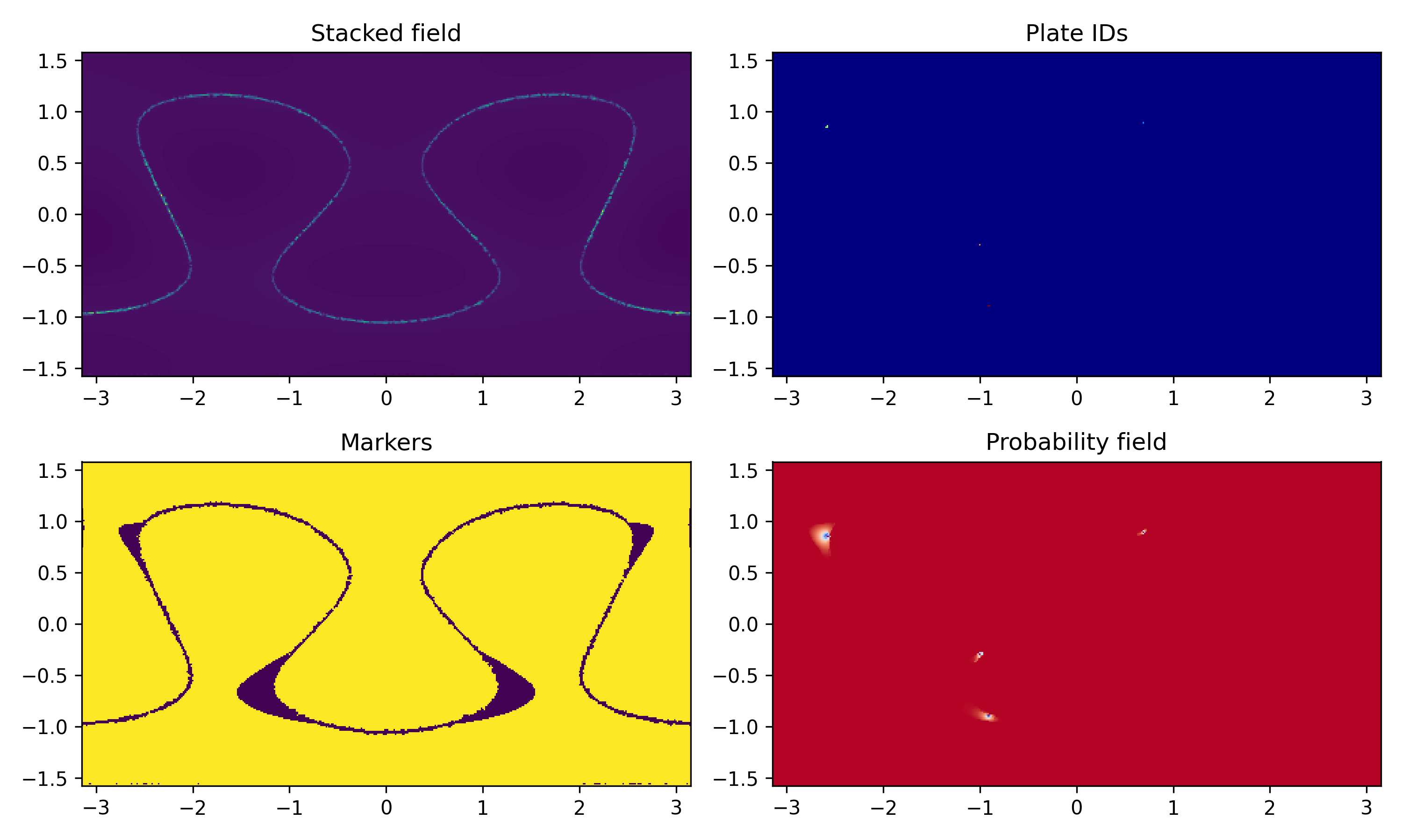
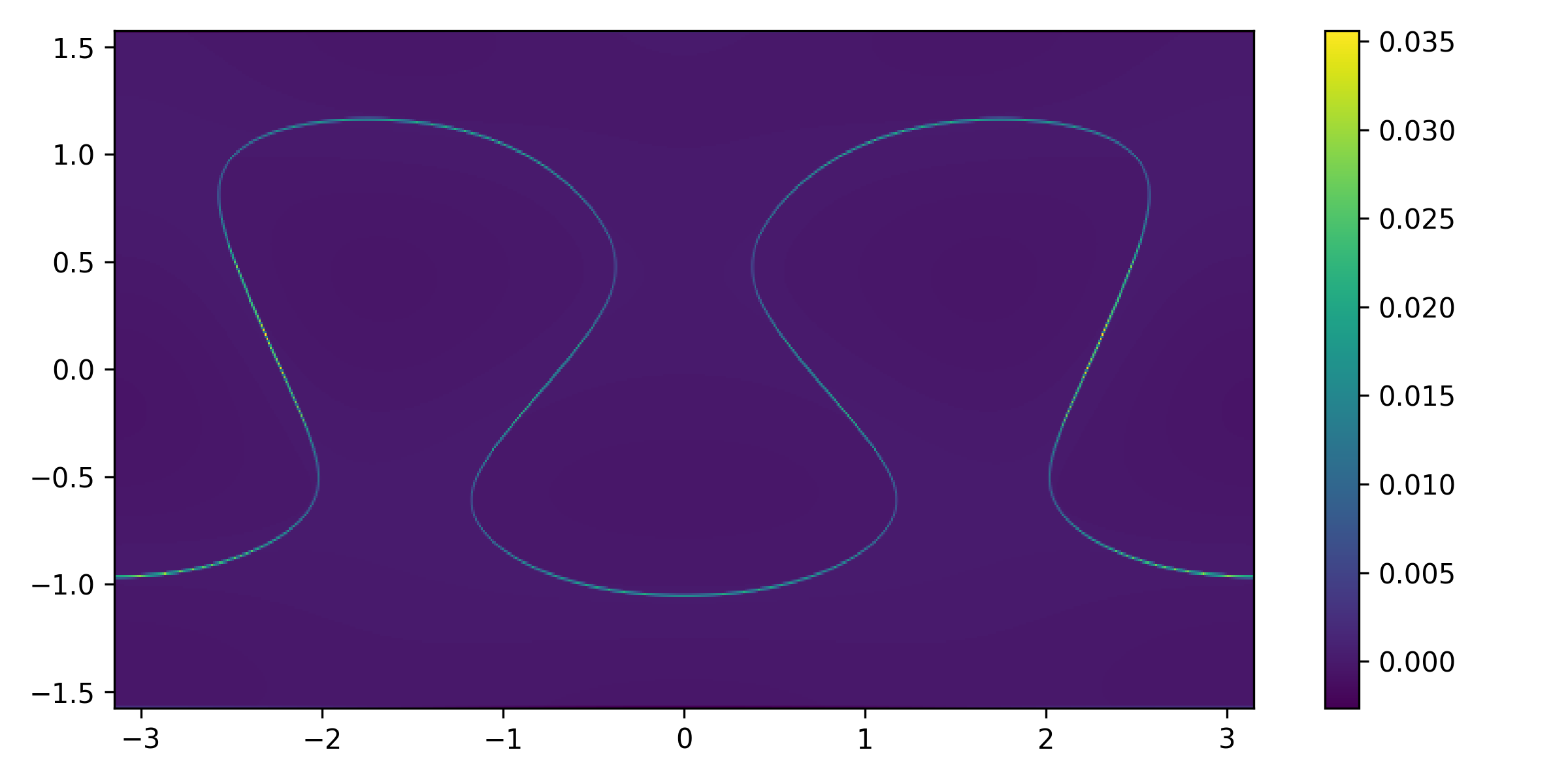
Looking at the plotted panels, we can see that seemingly no plates were detected.
This could be due to two main reasons:
-
boundary_quantile was set at too high of a value
-
Noisy input or missing boundary segments
This is why taking a look at model.markers (bottom left panel) is informative
as a diagnostic tool: it is clear that boundaries are well reflected on model.markers
which suggests the issue is not boundary_quantile. Rather, it is the noisy input
that has resulted in micro discontinuities along the boundary path. To remedy
this, we invoke separation_tolerance and set it at 1 degree:
| model.find_plates(
boundary_quantile = 0.95,
separation_tolerance = 1*np.pi/180, # in radians
RW_beta = 100.0,
)
|
or we can simply use platerecipy's built-in io functions:
| from platerecipy.io import save_mollweide_projection, save_as_vtk
# generating ParaView readable legacy .vtk
save_as_vtk(model)
# generating .png Mollweide projection
save_mollweide_projection(model)
|
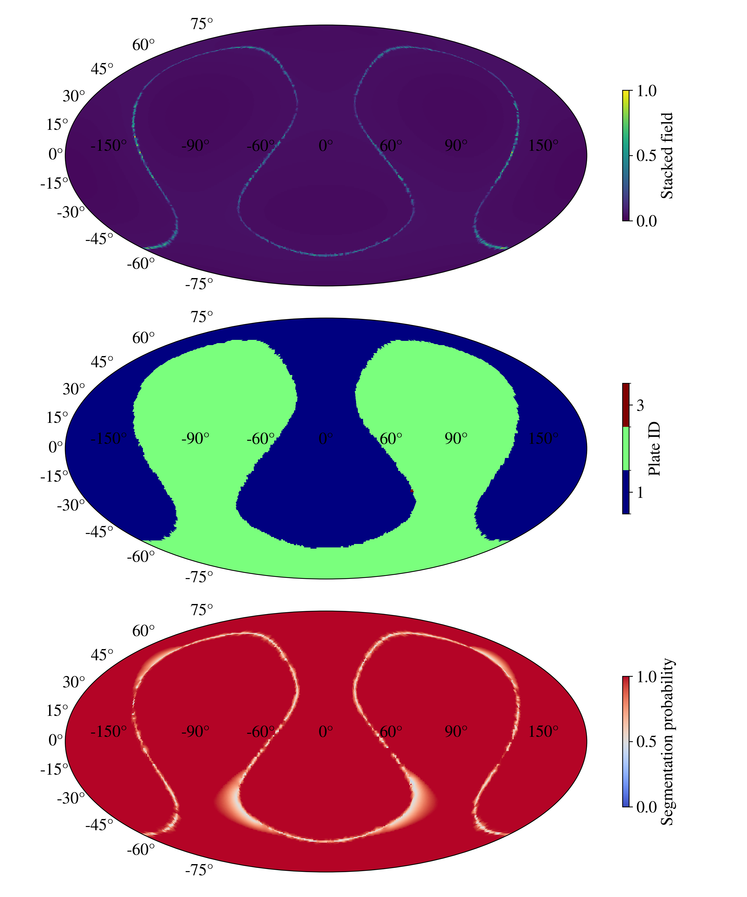
We can see that by introducing some separation tolerance, we were able to recover
the main candidate plates. The following subsection discusses the red micro marker (plate_ID == 3)
located roughly near 70 degrees east and 30 degrees south.
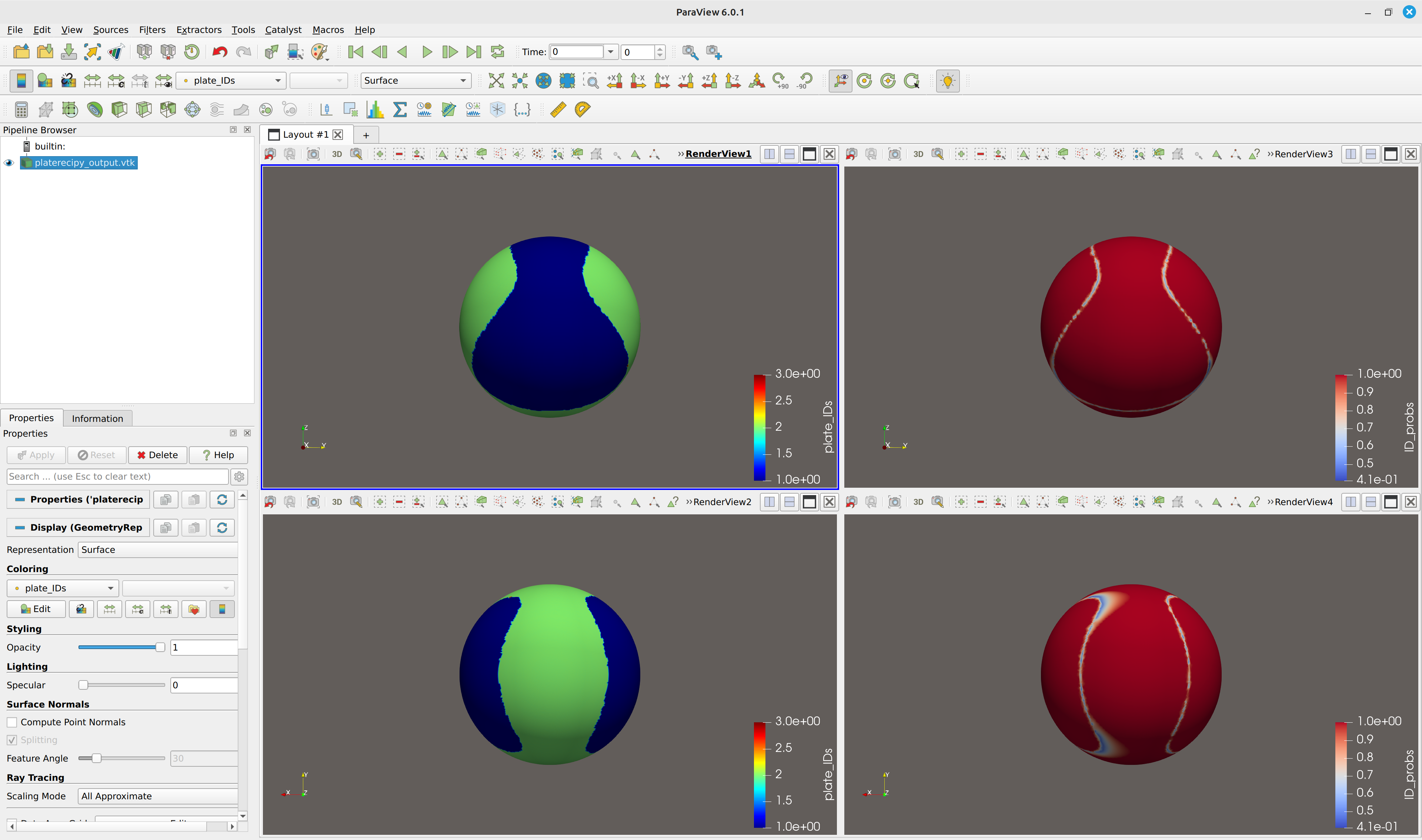
platerecipy.io.save_as_vtk vs. platerecipy.io.save_as_vtp
Both of these functions generate ParaView readable output. However, save_as_vtk
does not require third party packages of vtk and pyvista. Accordingly,
by default save_as_vtk is preferred.
Complete script (click)
1
2
3
4
5
6
7
8
9
10
11
12
13
14
15
16
17
18
19
20
21
22
23
24
25
26
27
28
29
30
31
32
33
34
35
36
37
38
39
40
41
42
43
44
45
46
47
48
49
50
51
52
53
54
55
56
57
58
59
60
61
62
63
64
65
66
67
68
69
70
71
72
73
74
75
76
77
78
79
80
81
82
83
84
85 | import numpy as np
def generate_sample_input(lrange=(1, 4), rng_seed=111, npoints=100_000):
from scipy.special import sph_harm_y
from scipy.ndimage import laplace
thetas, phis = np.meshgrid(
np.linspace(0, np.pi, 300),
np.linspace(-np.pi, np.pi, 600),
indexing='ij'
)
rng = np.random.default_rng(rng_seed)
F = 0
for l in range(lrange[0], lrange[1]):
for m in range(-l, l+1):
F += (rng.uniform()-0.25) * sph_harm_y(l, m, thetas, phis).real
F = laplace(np.abs(F))
rand_data = rng.choice(thetas.size, size=npoints, replace=False)
data_phis = phis.ravel()[rand_data]
data_thetas = thetas.ravel()[rand_data]
data_F = F.ravel()[rand_data]
data_xs = np.sin(data_thetas)*np.cos(data_phis)
data_ys = np.sin(data_thetas)*np.sin(data_phis)
data_zs = np.cos(data_thetas)
return data_xs, data_ys, data_zs, data_F
data_xs, data_ys, data_zs, data_F = generate_sample_input()
from platerecipy.grid import SphericalGrid

# initializing a grid base on input coordinates
grid = SphericalGrid(data_xs, data_ys, data_zs)

# interpolating the input data
field1 = grid.interpolate_field(data_F)
from platerecipy.model import PlateModel

# initializing a plate model
model = PlateModel(grid)

# stacking our interpolated field
model.stack_field(field1)

# additional fields can be stacked here
model.find_plates(
boundary_quantile = 0.95,
separation_tolerance = 1*np.pi/180.,
RW_beta = 100.0,
)
import matplotlib.pyplot as plt

fig, axes = plt.subplots(2, 2, figsize=(10, 6))

ax = axes[0][0]
ax.set_title("Stacked field")
ax.pcolormesh(grid.phis, np.pi/2 - grid.thetas, model.stacked_field)

ax = axes[1][0]
ax.set_title("Markers")
ax.pcolormesh(grid.phis, np.pi/2 - grid.thetas, model.markers)

ax = axes[0][1]
ax.set_title("Plate IDs")
ax.pcolormesh(grid.phis, np.pi/2 - grid.thetas, model.plate_IDs, cmap="jet")

ax = axes[1][1]
ax.set_title("Probability field")
ax.pcolormesh(grid.phis, np.pi/2 - grid.thetas, model.ID_probs, cmap="coolwarm")

fig.tight_layout()
fig.savefig("field_plots.png", dpi=300)
from platerecipy.io import save_mollweide_projection, save_as_vtk

# generating ParaView readable legacy .vtk
save_as_vtk(model)

# generating .png Mollweide projection
save_mollweide_projection(model)
|
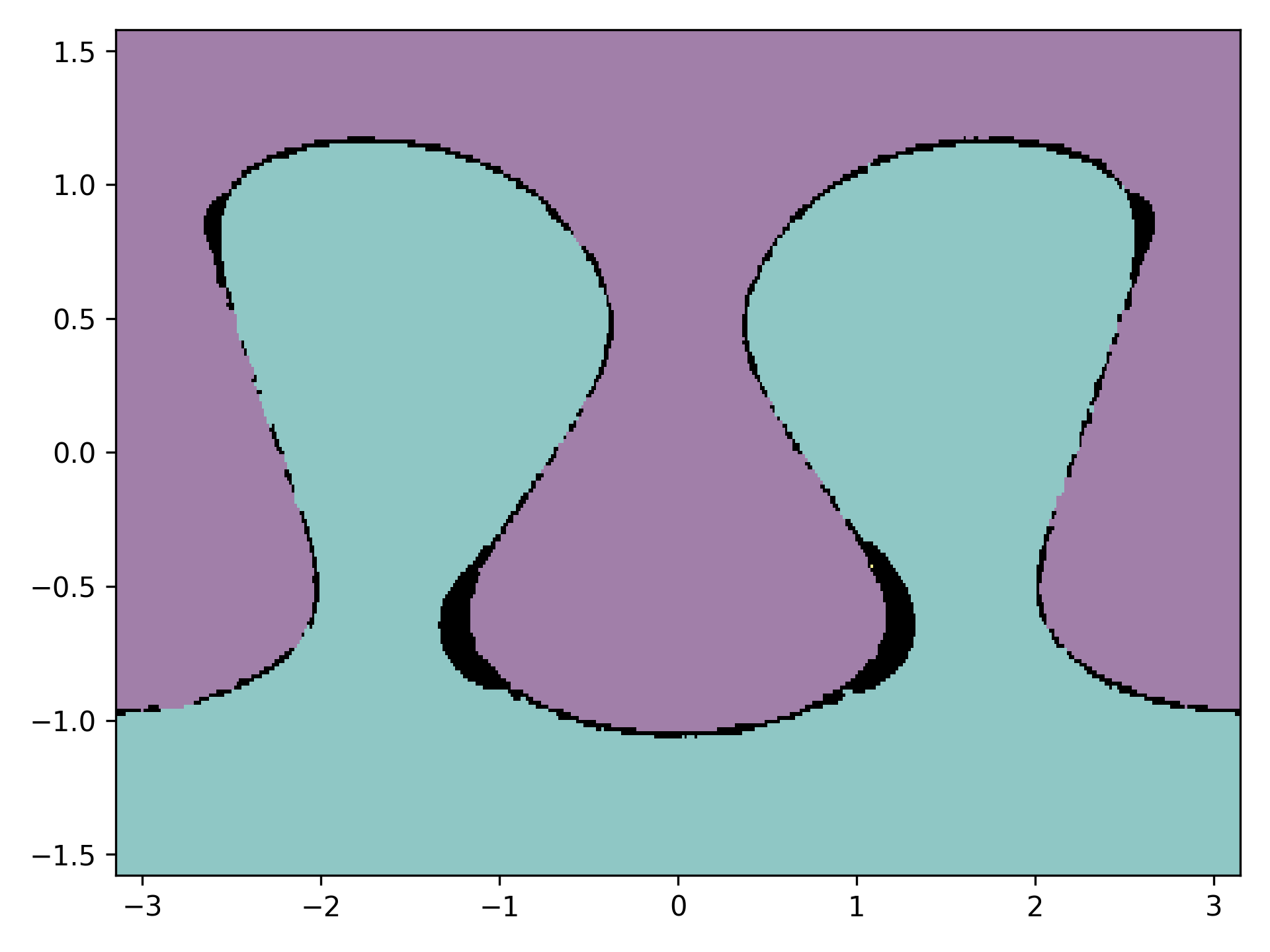
Micro markers and noise
In noisy or low resolution input, it is possible to end up with a very small set of
nodes clump together and generate fictitious micro markers. Our example above
illustrates this problem: at the boundary of plates 1 and 2, there are a few
nodes near 70 degrees east and 30 degrees south that gave rise to a distinct (micro)
marker that resulted in those nodes getting assigned plate ID 3.
In these scenarios, it is useful to invoke min_marker_size argument to filter
markers comprised of fewer than a given number of points.
Having access to the probability field in addition to the stacked field allows
us to identify low-confidence and/or diffuse regions which we will refer to them
here as non-conforming regions.
numpy array indexing allows for an easy and straight forward way of identifying
such regions. In our example with two plates, we can search for regions with
an ID assignment probability of less than 80 percent:
| # plotting the plate IDs
plt.pcolormesh(grid.phis, np.pi/2-grid.thetas, model.plate_IDs, alpha=0.5)
# plotting low-confidence regions in black shading
temp = model.ID_probs.copy()
temp[(model.ID_probs > 0.8)] = float('NaN')
plt.pcolormesh(grid.phis, np.pi/2-grid.thetas, temp, cmap='Grays', vmin=-1, vmax=0)
|
We can map any field of our choice back to the input by calling:
| org_IDs = grid.map_to_original_input(model.plate_IDs)
|
and plotting the data points:
| plt.scatter(grid.original_phis, np.pi/2 - grid.original_thetas, c=org_IDs, marker='.', s=0.1)
|